Introduction
The National Hockey League (NHL) is considered to be the premier professional ice hockey league in the world, founded 102 years ago in 1917. Like many other sports, the data about teams, players, games, and more are a great resource to dive in and analyze using modern software tools. Thanks to the open NHL API, the data is accessible to everyone and the {nhlapi} R package aims to make that data readily available for analysis to R users.
In this post, we will use the
{nhlapi}R package to explore the positional data on in-game events, which will provide us with information on the plays that happened in matches and where they happened in terms of the position on the rink. We will also show ways to plot that information using 2D density charts with{ggplot2}.
Contents
Installing the {nhlapi} package
We can install {nhlapi} from CRAN. It has only 1 recursive dependency, so the installation is very light and swift. Alternatively, we can also install the latest development version from the master branch on GitHub using the {remotes} or {devtools} package:
# Current CRAN version:
install.packages("nhlapi")

# Development version from GitHub
#  devtools::install_github("jozefhajnala/nhlapi")
#  remotes::install_github("jozefhajnala/nhlapi")

library(nhlapi)
Now we attach the package using library() or require() and can start exploring the data. All the relevant functions start with the nhl_ prefix so they are easy to find and are well documented, so we can get help by using the help() function in R. For example, in this post we will look at the detailed games’ data, so running help(nhl_games) will provide us with detailed information on the available functions.
Retrieving basic game information
To look at a quick example, we will explore the very first game in the regular season 2017/2018, in which the Toronto Maple Leafs played against the Winnipeg Jets. First, let’s look at the very basic game results using the nhl_games_linescore() function which retrieves a very limited amount of high-level information:
linescore <- nhlapi::nhl_games_linescore(gameIds = 2017020001)[[1]]

# Look at quick info on periods
linescore$periods
periodType startTime endTime num ordinalNum
1 REGULAR 2017-10-04T23:17:19Z 2017-10-04T23:58:23Z 1 1st
2 REGULAR 2017-10-05T00:16:56Z 2017-10-05T00:54:10Z 2 2nd
3 REGULAR 2017-10-05T01:12:37Z 2017-10-05T01:50:38Z 3 3rd
home.goals home.shotsOnGoal home.rinkSide away.goals away.shotsOnGoal
1 0 17 right 3 11
2 0 10 left 1 8
3 2 10 right 3 12
away.rinkSide
1 left
2 right
3 leftGetting detailed events data for a game
Now to something more interesting, lets investigate what plays were made during the game and where on the ice they happened. We can use nhl_games_feed() to get the most detailed game data available in the API. To get a picture of the amount of detail, we can print the structure of the retrieved object limited to 3 levels of depth:
gameIds <- 2017020001
gameFeed <- nhlapi::nhl_games_feed(gameIds = gameIds)[[1]]
str(gameFeed, max.level = 3)
List of 6
$ copyright: chr "NHL and the NHL Shield are registered trademarks of the National Hockey League. NHL and NHL team marks are the "| __truncated__
$ gamePk : int 2017020001
$ link : chr "/api/v1/game/2017020001/feed/live"
$ metaData :List of 2
..$ wait : int 10
..$ timeStamp: chr "20171006_173713"
$ gameData :List of 6
..$ game :List of 3
.. ..$ pk : int 2017020001
.. ..$ season: chr "20172018"
.. ..$ type : chr "R"
..$ datetime:List of 2
.. ..$ dateTime : chr "2017-10-04T23:00:00Z"
.. ..$ endDateTime: chr "2017-10-05T01:50:41Z"
..$ status :List of 5
.. ..$ abstractGameState: chr "Final"
.. ..$ codedGameState : chr "7"
.. ..$ detailedState : chr "Final"
.. ..$ statusCode : chr "7"
.. ..$ startTimeTBD : logi FALSE
..$ teams :List of 2
.. ..$ away:List of 16
.. ..$ home:List of 16
..$ players :List of 45
.. ..$ ID8474709:List of 22
.. ..$ ID8473618:List of 22
.. ..$ ID8471218:List of 22
.. ..$ ID8470828:List of 21
.. ..$ ID8477939:List of 22
.. ..$ ID8476945:List of 22
.. ..$ ID8473412:List of 22
.. ..$ ID8475716:List of 21
.. ..$ ID8476941:List of 22
.. ..$ ID8476469:List of 21
.. ..$ ID8477359:List of 22
.. ..$ ID8479339:List of 21
.. ..$ ID8479318:List of 22
.. ..$ ID8476410:List of 22
.. ..$ ID8475883:List of 21
.. ..$ ID8474574:List of 22
.. ..$ ID8477940:List of 21
.. ..$ ID8473463:List of 21
.. ..$ ID8477464:List of 22
.. ..$ ID8473461:List of 22
.. ..$ ID8476392:List of 22
.. ..$ ID8466139:List of 22
.. ..$ ID8470834:List of 22
.. ..$ ID8468575:List of 22
.. ..$ ID8477429:List of 22
.. ..$ ID8468493:List of 22
.. ..$ ID8474037:List of 22
.. ..$ ID8475786:List of 22
.. ..$ ID8470611:List of 22
.. ..$ ID8476853:List of 22
.. ..$ ID8477448:List of 21
.. ..$ ID8477504:List of 22
.. ..$ ID8479458:List of 21
.. ..$ ID8477015:List of 22
.. ..$ ID8475179:List of 21
.. ..$ ID8476885:List of 22
.. ..$ ID8475279:List of 22
.. ..$ ID8473574:List of 22
.. ..$ ID8476460:List of 22
.. ..$ ID8475098:List of 22
.. ..$ ID8474581:List of 22
.. ..$ ID8478483:List of 22
.. ..$ ID8475172:List of 22
.. ..$ ID8480158:List of 21
.. ..$ ID8479293:List of 22
..$ venue :List of 3
.. ..$ id : int 5058
.. ..$ name: chr "Bell MTS Place"
.. ..$ link: chr "/api/v1/venues/5058"
$ liveData :List of 4
..$ plays :List of 5
.. ..$ allPlays :'data.frame': 312 obs. of 28 variables:
.. ..$ scoringPlays : int [1:9] 93 108 112 157 225 269 284 286 290
.. ..$ penaltyPlays : int [1:12] 21 43 66 86 117 148 167 183 247 253 ...
.. ..$ playsByPeriod:'data.frame': 3 obs. of 3 variables:
.. ..$ currentPlay :List of 3
..$ linescore:List of 10
.. ..$ currentPeriod : int 3
.. ..$ currentPeriodOrdinal : chr "3rd"
.. ..$ currentPeriodTimeRemaining: chr "Final"
.. ..$ periods :'data.frame': 3 obs. of 11 variables:
.. ..$ shootoutInfo :List of 2
.. ..$ teams :List of 2
.. ..$ powerPlayStrength : chr "Even"
.. ..$ hasShootout : logi FALSE
.. ..$ intermissionInfo :List of 3
.. ..$ powerPlayInfo :List of 3
..$ boxscore :List of 2
.. ..$ teams :List of 2
.. ..$ officials:'data.frame': 4 obs. of 4 variables:
..$ decisions:List of 5
.. ..$ winner :List of 3
.. ..$ loser :List of 3
.. ..$ firstStar :List of 3
.. ..$ secondStar:List of 3
.. ..$ thirdStar :List of 3
- attr(*, "url")= chr "https://statsapi.web.nhl.com/api/v1/game/2017020001/feed/live"Now lets finally look at the data on plays. We can access those via the allPlays data.frame inside the element plays of liveData. The below code chunk will store those in a separate data.frame called plays. We can then filter based on result.event to look for instance only at goals.
plays <- gameFeed$liveData$plays$allPlays
goals <- plays[plays$result.event == "Goal", ]

# Selecting limited columns to keep the print reasonable
goals[, c(2, 5, 6, 12, 15, 18, 26, 23, 24)]
## result.event
## 94 Goal
## 109 Goal
## 113 Goal
## 158 Goal
## 226 Goal
## 270 Goal
## 285 Goal
## 287 Goal
## 291 Goal
## result.description
## 94 Nazem Kadri (1) Wrist Shot, assists: James van Riemsdyk (1), Tyler Bozak (1)
## 109 James van Riemsdyk (1) Wrist Shot, assists: Tyler Bozak (2)
## 113 William Nylander (1) Wrist Shot, assists: Jake Gardiner (1), Auston Matthews (1)
## 158 Patrick Marleau (1) Backhand, assists: Auston Matthews (2), Mitchell Marner (1)
## 226 Patrick Marleau (2) Wrist Shot, assists: Nazem Kadri (1), Leo Komarov (1)
## 270 Mitchell Marner (1) Wrist Shot, assists: James van Riemsdyk (2), Morgan Rielly (1)
## 285 Mark Scheifele (1) Snap Shot, assists: Patrik Laine (1), Dustin Byfuglien (1)
## 287 Auston Matthews (1) Tip-In, assists: Connor Carrick (1), Andreas Borgman (1)
## 291 Mathieu Perreault (1) Wrist Shot, assists: Bryan Little (1)
## result.secondaryType result.strength.name about.period
## 94 Wrist Shot Power Play 1
## 109 Wrist Shot Even 1
## 113 Wrist Shot Even 1
## 158 Backhand Even 2
## 226 Wrist Shot Even 3
## 270 Wrist Shot Power Play 3
## 285 Snap Shot Even 3
## 287 Tip-In Even 3
## 291 Wrist Shot Even 3
## about.periodTime team.name coordinates.x coordinates.y
## 94 15:45 Toronto Maple Leafs 84 -6
## 109 17:40 Toronto Maple Leafs 62 5
## 113 18:23 Toronto Maple Leafs 84 -22
## 158 08:32 Toronto Maple Leafs -82 2
## 226 00:36 Toronto Maple Leafs 68 12
## 270 08:07 Toronto Maple Leafs 85 -6
## 285 11:31 Winnipeg Jets -82 8
## 287 11:57 Toronto Maple Leafs 84 -3
## 291 12:57 Winnipeg Jets -80 1Now we can see that there are many columns, among them coordinates.x and coordinates.y which tell us the location of the play on the rink, where [0, 0] is the center of the rink.
More involved data retrieval - many games in parallel
Now we know how to look at the positional data for one match so one very interesting aspect of the data is where plays happen overall. We will now investigate and plot where different plays were happening in the regular season 2017/2018. Looking at ?nhl_games we see that for regular seasons we can usually get all the gameIds in the interval 2017020001:2017021271.
# Define the game ids
gameIds <- 2017020001:2017021271

# Retrieve the data
gameFeeds <- nhlapi::nhl_games_feed(gameIds)
To retrieve the data a bit faster, we can also use the parallel package which is part of the base R installation to retrieve the data in parallel, for example, like so.
# Define the game ids
gameIds <- 2017020001:2017021271

# Create a local cluster
cl <- parallel::makeCluster(parallel::detectCores() / 2)

# Retrieve the data using nhlapi::nhl_games_feed()
gameFeeds <- parallel::parLapplyLB(cl, gameIds, nhlapi::nhl_games_feed)

# Stop the cluster
parallel::stopCluster(cl)
Now we have the data retrieved in a list called gameFeeds. It might be wise to store it on disk such that we do not have to do the long retrieval all the time, for example using saveRDS():
saveRDS(gameFeeds, file.path("~", "gamefeeds_regular_2017.rds"))Processing and plotting positional data
Now that the data is safely retrieved, we can process and prepare the data on plays for plotting.
# Retrieve the data frames with plays from the data
getPlaysDf <- function(gm) {
playsRes <- try(gm[[1L]][["liveData"]][["plays"]][["allPlays"]])
if (inherits(playsRes, "try-error")) data.frame() else playsRes
}
plays <- lapply(gameFeeds, getPlaysDf)
# Bind the list into a single data frame
plays <- nhlapi:::util_rbindlist(plays)
# Keep only the records that have coordinates
plays <- plays[!is.na(plays$coordinates.x), ]
# Move the coordinates to non-negative values before plotting
plays$coordx <- plays$coordinates.x + abs(min(plays$coordinates.x))
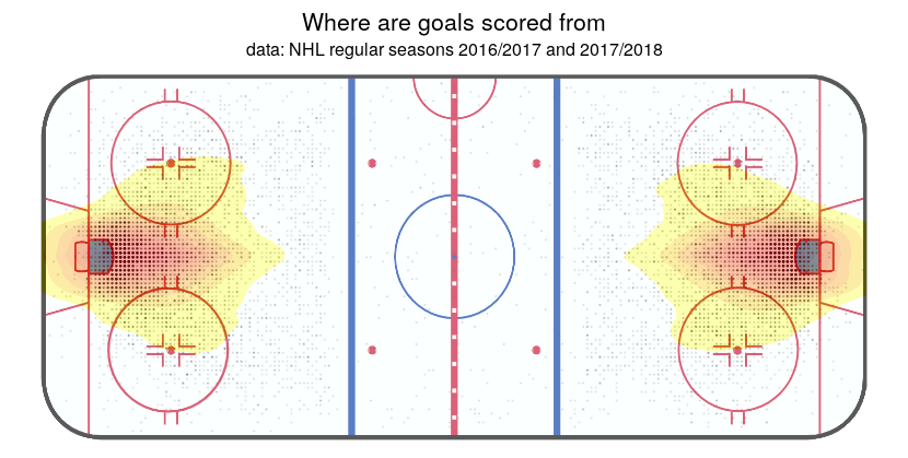
plays$coordy <- plays$coordinates.y + abs(min(plays$coordinates.y))Now we have the data ready in a plays data.frame, finally we can create some cool plots. As an example, in the following chunk the popular ggplot2 package is used to plot densities and events that would yield results similar to the ones shown below:
library(ggplot2)

# Look at goals only
goals <- plays[result.event == "Goal"]

ggplot(goals, aes(x = coordx, y = coordy)) +
  labs(title = "Where are goals scored from") +
  geom_point(alpha = 0.1, size = 0.2) +
  xlim(0, 198) + ylim(0, 84) +
  geom_density_2d_filled(alpha = 0.35, show.legend = FALSE) +
  theme_void()
Some examples of rendered images
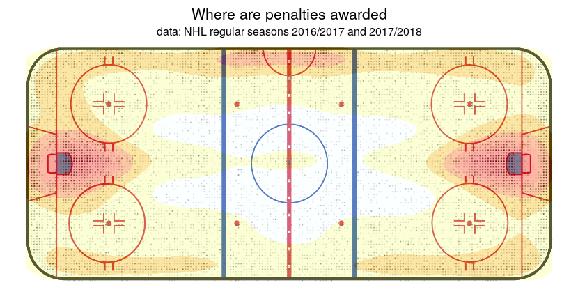
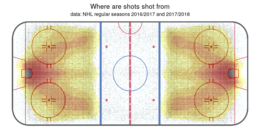
With a bit of effort, we can also add a background image of the ice hockey rink to make the density plots more relatable and arrive at some quite informative plots:
Happy exploring!
References
- The
{nhlapi}package on CRAN - The
{nhlapi}package on GitHub