Introduction
In this post we will look at yet another productivity increasing feature of the RStudio IDE - Code Snippets. Code Snippets let us easily insert and potentially execute predefined pieces of code and work not just for R code, but many other languages as well.
In this post we will cover 4 different ways to increase productivity using Code Snippets and provide 11 real-life examples of their use that you can take advantage of instantly.
How do Code Snippets work
Using, Viewing and editing snippets
- In RStudio, we can browse and define snippets under
Tools -> Global Options... -> Code -> Edit Snippetswindow - When typing code, the snippet will appear as an auto-complete option (similar to function names) if we type the first few letters of its name
- Use
Shift+Tabto insert the snippet immediately or pick the snippet from the auto-complete list (by clicking or scrolling on it and pressingTab)
Note that as there is no auto-completion when editing R Markdown documents, we need to use the
Shift+Tabmethod exclusively in that case.
Four common use-case scenarios
1. Automatically insert boilerplate or template-style code
The first and probably most frequent use of the Code Snippets feature is to quickly insert predefined pieces of code that require a lot of typing with little alternation, a.k.a. boilerplate code. A good illustration is a snippet covering a tryCatch block:
snippet tryc
    ${1:variable} <- tryCatch({
        ${2}
    }, warning = function(w) {
        message(sprintf("Warning in %s: %s", deparse(w[["call"]]), w[["message"]]))
        ${3}
    }, error = function(e) {
        message(sprintf("Error in %s: %s", deparse(e[["call"]]), e[["message"]]))
        ${4}
    }, finally = {
        ${5}
    })
Note that the snippet definition is intended using
<tab>instead of spaces.
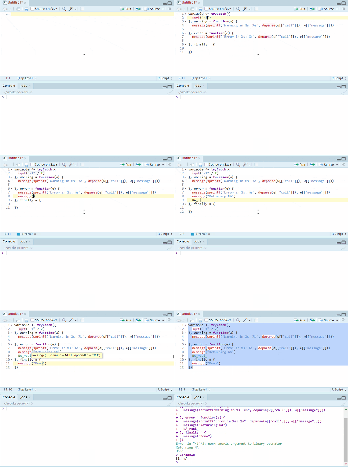
After defining this Snippet and running it we will automatically get a good template for the block and we can focus on writing the important parts:

The numbered sections prefixed with
$such as${2}let us define sections to which the cursor will jump after pressingTab. We can also use${1:predefinedvalue}to predefine a value for the sections.
Another example of this type of use may be a testthat block that quickly prepares a unit-testing file:
snippet tt
    context("${1}")

    # ${2} ----------
    test_that(
      "${2}",
      expect_${3}(${4})
    )
2. Pre-fill code to be ran quickly
The second use case scenario where the Code Snippets come in really handy is to use them in the console when we want to run a block of code that we execute often in some scenarios. One such example is to attach the packages we use in a particular context. For example, when developing an R package, the following may be handy:
snippet dd
    "library('devtools'); library('testthat'); library('pryr')"
With this snippet, after pressing dd and then Shift+Tab in the console, the library statements will appear and we can just press enter to run them and attach the mentioned packages. We can of course make separate snippets for example for attaching packages we use for interactive data analysis and plotting. This is one way to keep our .Rprofile clean and still have packages easily available when needed.
Another example for this scenario is to quickly run a benchmark comparing two or more pieces of code and visualize the results with a boxplot to get an overview:
snippet mm
    bench <- microbenchmark::microbenchmark(
        times = ${1:1:100},
        ${2:one} = ${3},
        ${4:two} = ${5}
        )
    if (requireNamespace("highcharter")) {
      highcharter::hcboxplot(bench[["time"]], bench[["expr"]], outliers = FALSE)
    } else {
      boxplot(bench, outline = FALSE)
    }
3. Execute code combined with rstudioapi
The one scenario where RStudio really shines is combining multiple features it offers. We can neatly combine the use of snippets, rstudioapi and the Terminal feature that we discussed previously for an amazing variety of productivity boosts.
Just one practical example convenient when writing a blogdown site is to instantly serve a preview of the blog in a separate session via the Terminal and use the RStudio Viewer in one go to view the site. This is handy especially in the RStudio Server setting, where the site serving in the same session can make the IDE behave slow:
snippet ss
    `r eval({
      nocon <- function(link = 'http://127.0.0.1:9999') {
        inherits(suppressWarnings(try({
            con <- url(link, open = 'rb')
            close(con)
        }, silent = TRUE)), 'try-error')
      }
      if (nocon()) {
        termId <- rstudioapi::terminalExecute(
          'R -q -e \"blogdown::serve_site(port = 9999,  browser = FALSE)\"',
          show = FALSE
        )
        while (nocon() && !identical(rstudioapi::terminalExitCode(termId), 1L)) {
            Sys.sleep(0.25)
            cat(".")
        }
      }
      if (identical(rstudioapi::terminalExitCode(termId), 1L)) {
        cat(rstudioapi::terminalBuffer(termId), sep = "\n")
      } else {
        rstudioapi::viewer('http://127.0.0.1:9999')
      }
    })`
After pressing ss and Shift+Tab, the site will be served in a separate R Session and previewed in the viewer.
Using
eval(expression)like above lets us execute R code in snippets. This gives a lot of flexibility, even more extensive when combined witheval(parse(text = "code as character string"))
4. Execute code and paste result at cursor
The fourth option is to inject text following the cursor using $$. An example simple but potentially powerful use of this feature is to pass commands to be executed via base R’s system and getting the results directly at our cursor:
snippet $$
    `r eval(parse(text = "system('$$', intern = TRUE)"))`
With the above, when typing $$ls into the editor and pressing Shift+Tab, we will see the list of files present in our working directory placed at our cursor.
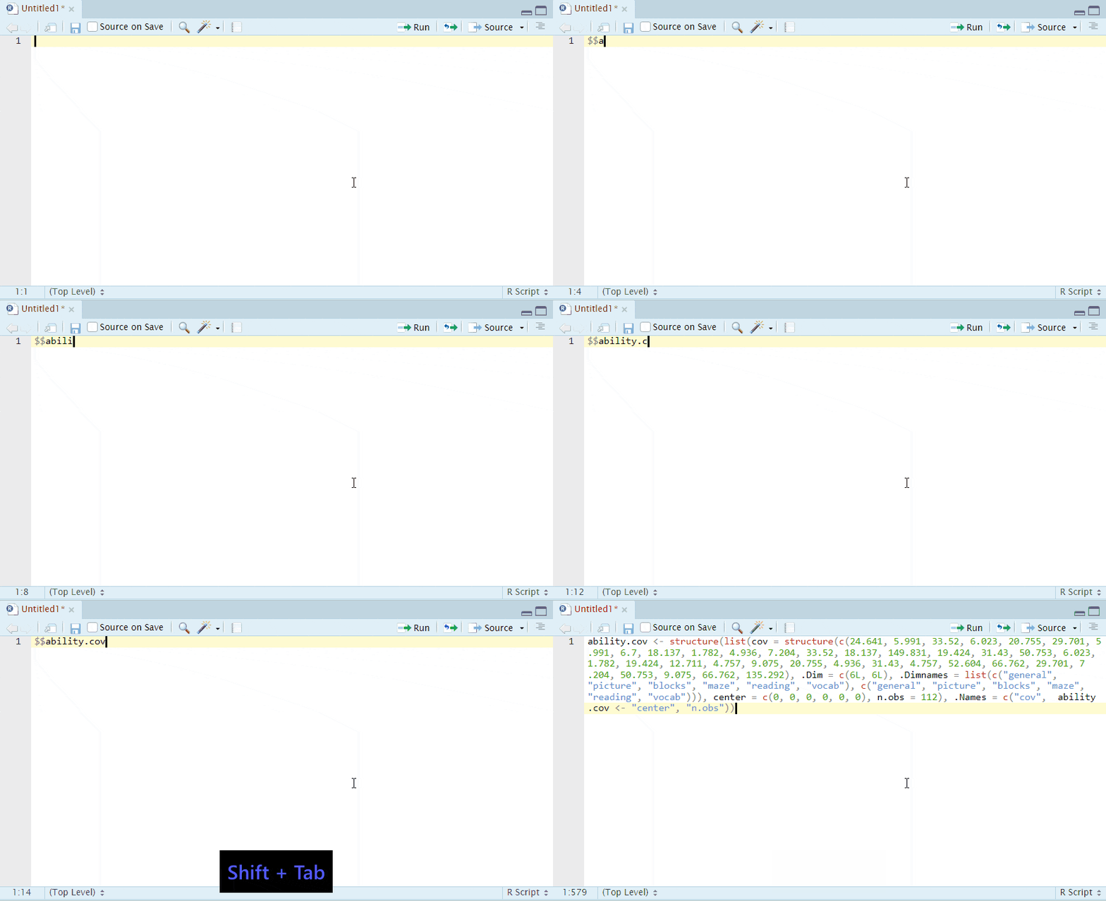
Another handy use of this feature is to be able to quickly get a reproducible object definition by deparsing it:
snippet $$
    `r paste("$$ <-", deparse(eval(parse(text="$$")), width.cutoff = 500L))`
TL;DR - Just give me the snippets
The promised 11 potentially helpful snippets can be found here.
Resources
- Code Snippets by J.J. Allaire at the RStudio support
- 4 ways to be more productive, using RStudio’s terminal