Introduction
Including R Markdown in the workflow for presenting and publishing analyses that use code in R or other languages is a great way to make presentations, dashboards or reports good looking, reproducible and version controllable.
In this post, we will look at three simple ways to improve that workflow even further with methods that are lesser known and can make producing results with R Markdown more efficient and reviewing them more interactive.
Contents
Live preview of R Markdown files with xaringan’s infinite_moon_reader()
If you are familiar with R notebooks, you probably know that as you edit the notebook in RStudio and save, the preview will automatically update in the RStudio viewer. Similarly for blogdown users, the serve_site() function provides live updates of the blog as the content is edited and saved.
However, if you are producing presentation slides or a more complex html report with R Markdown, you are stuck with re-knitting every time you want to see the updated content in action. Enter the
infinite_moon_reader()function from the xaringan package.
Even though the xaringan package focuses on creating slides with the remark.js JavaScript library, this function works to provide a live preview with any single-file html output, be it a report, slides such as ioslides, a shiny document or another format.
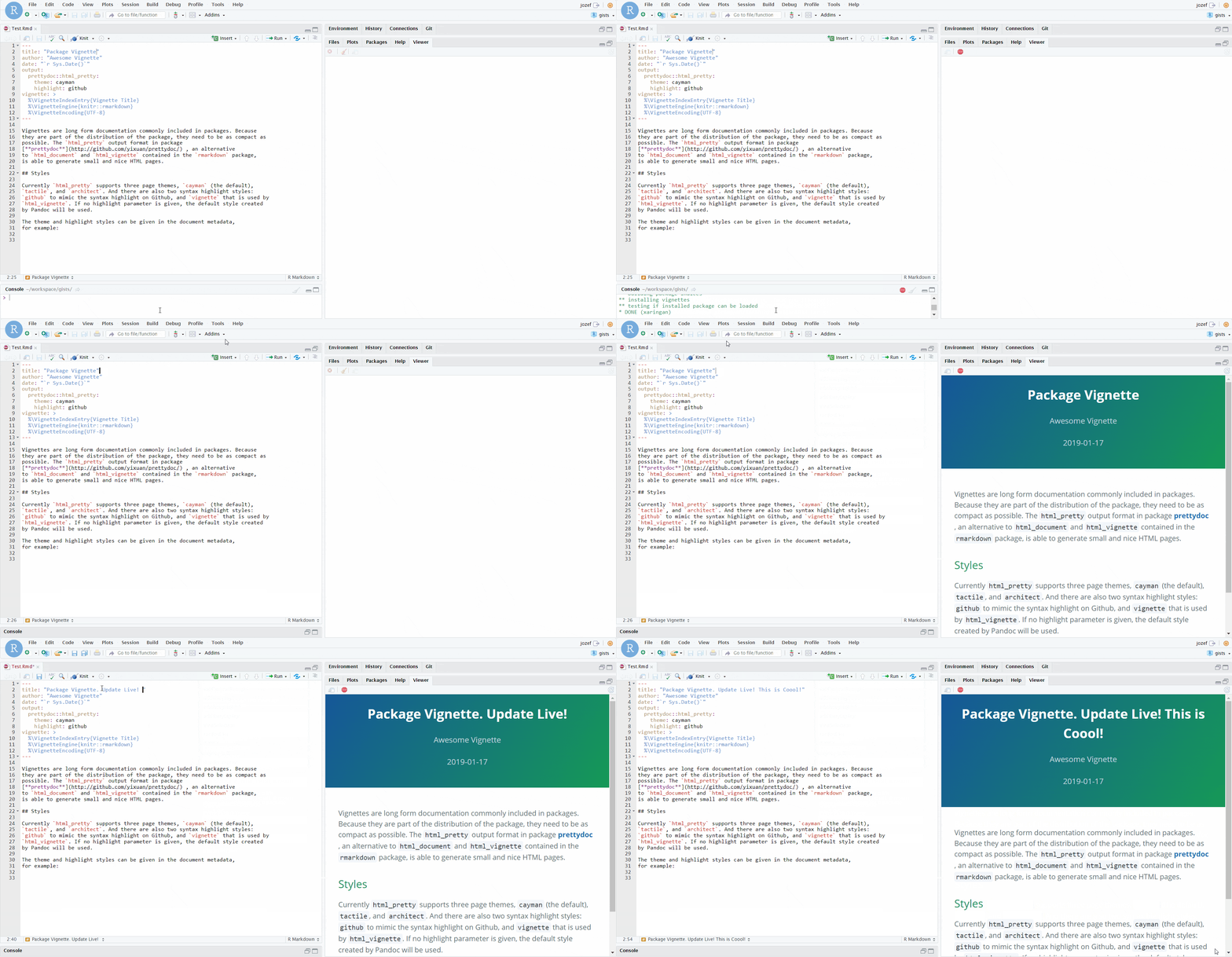
If using RStudio, all you need to do to get the live preview is call the function and the default values of the arguments will take care of launching the live preview of the document currently active in the RStudio editor. As if this was not handy enough, the package comes with a premade RStudio addin, so you can get the same functionality just clicking in the IDE, or assigning a keyboard shortcut to it.
It is really that easy
Here is how long it takes to get it up and running, package installation included:

Infinite moon reader
Kind of obviously, this functionality can become a huge time saver, especially if you are tweaking the design of your slides and want to see the results quickly without the need to click/call knit over and over again.
Creating beautiful, multi format reports directly from R scripts
When creating R Markdown documents, the workflow often looks something like the following:
- Create a new .Rmd file, edit the metadata
- Write some content
- Add code chunks, test
- Write some more content
- Add some more code chunks, test
- Rinse and repeat
This works, but when your goal is to first create functioning code that you can run as-is and share with others, creating an R Markdown file from such a script with that approach can become a time consuming and error-prone process of copy-pasting the code into code chunks and maintaining it in two places in case you want to also keep the runnable script version.
In comes knitr’s
spin()
The solution to the above problem is very simple once you are aware of it. You can use knitr’s spin() function to produce a beautiful report directly from an R script, with advanced formatting and options still being available - via formatted comments and the function’s parameters.
This way we can keep the script fully runnable as comments do not interfere with running the code, and still be able to produce that nice output R Markdown is known for.
A quick example
A working example is worth more than explanations here, so here we go. Just copy the following, save for example into script.R and run knitr::spin("script.R"):
#' # This is just an R script
#' ## Rendered to a html report with knitr::spin()
#' * just by adding comments we can make a really nice output

#'
#' > And the code runs just like normal, eg. via `Rscript` after all
#' __comments__ are just *comments*.
#'
#' ## The report begins here
#+
knitr::kable(head(mtcars))

#' ## A chart
#+ fig.width=8, fig.height=8
heatmap(cor(mtcars))

#' ## Some tips
#'
#' 1. Optional chunk options are written using `#+`
#' 1. You can write comments between `/*` and `*/`
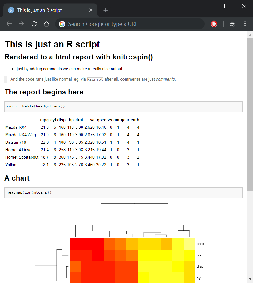
By default, the result will something like the following:

Spinned it right round
Compile Report and RMarkdown’s render() vs. knitr’s spin()
We can achieve similar results in RStudio by clicking on File -> Compile Report..., which is equivalent to using rmarkdown::render() on an R script file. This will call spin() and add some metadata such as title, author and time to the output.
So why bother with
spin()at all?
The default behavior has some important differences between calling the functions mentioned above. One of them for HTML output is that render() will by default include inline base64 representations of fonts and JavaScript sources, increasing the output file size from less them 20 KB to more than 600 KB even with the smallest amount of content.
This is why I personally like to call knitr::spin() to keep the output at smaller sizes by default, without having to dig in into the options passed to pandoc.
Regardless of the technical details, being able to produce good looking reports directly from R scripts can save a lot of time and error-prone copying, while keeping the content and runnable code in one place, instead of copy-pasting into code chunks of an R Markdown file.
This is of course not to say that R Markdown files are not useful. To the contrary, they are great for many use cases. However, if the content is mostly code with some accompanying text, using spin() can come in really handy.
Advanced chunk options with useful effects
When working with R Markdown the code chunk options provide helpful modifications to the chunk code’s behavior. The simple and widely used chunk options such as the following are well known, we mention them for a quick reference:
eval=FALSE- do not evaluate the code in the chunk at allecho=FALSE- do not show the chunk code in the output fileinclude=FALSE- do not show code output in the output filemessage=FALSE- do not show messages in the output filewarning=FALSE- do not show warnings in the output fileerror=TRUE- do not prevent rendering on error and show error messages in the output
results='asis' to keep content generated by a chunk unprocessed
Especially when producing HTML output it may be helpful to create functions that produce output we want to include directly in the rendered document without any processing, such as HTML code produced by a pre-made function.
One example I use often is a function makeHighChart() that creates a lightweight JavaScript representation of a chart created via highcharter from an R object. The output of that function is HTML code that should be placed as-is into the output, for which the results='as-is' chunk option is made:
# This chunk uses the results='as-is' option like so:
# ```{r results='asis'}
# The results is an interactive chart:
jhaddins::makeHighChart(
  highcharter::hcboxplot(mtcars$hp),
  chartname = "examplechart",
  docat = TRUE
)
# This one does not use the results option, it is just
# ```{r}
# The result is not very useful printed HTML:
jhaddins::makeHighChart(
highcharter::hcboxplot(mtcars$mpg),
chartname = "examplechart",
docat = TRUE
)## <script type="text/javascript">
## $(function () {
## $('#examplechart').highcharts({
## title: {
## text: null
## },
## yAxis: {
## title: {
## text: null
## }
## },
## credits: {
## enabled: false
## },
## exporting: {
## enabled: false
## },
## plotOptions: {
## series: {
## label: {
## enabled: false
## },
## turboThreshold: 0,
## marker: {
## symbol: "circle"
## },
## showInLegend: false
## },
## treemap: {
## layoutAlgorithm: "squarified"
## }
## },
## chart: {
## type: "bar"
## },
## xAxis: {
## type: "category",
## categories: ""
## },
## series: [
## {
## name: null,
## data: [
## {
## name: null,
## low: 10.4,
## q1: 15.35,
## median: 19.2,
## q3: 22.8,
## high: 33.9
## }
## ],
## type: "boxplot",
## id: null
## }
## ]
## }
## );
## });
## </script>
##
## <div id="examplechart"></div>class.output="some_css_class" to format chunk output with custom css
For HTML output, we may want to style it with our own css. This option allows to use defined css classes to style the output produced by that chunk. This can be very convenient if we want to style some chunks in a different manner elegantly. We can also provide multiple css classes in a character vector instead of just one.
cache=TRUE to render faster and more reproducibly
In case your documents contain calculations that a take lot of time, or just cause unnecessary pain when re-executed with each render, for example when including benchmarking results in posts, it is very convenient to cache the chunk results. This will not only make the rendering faster, but also ensure that the results of the same code will stay the same in the output, even if we re-render the document.
Note that for keeping reproducibility when random number generation is included with caching results, it is advised to also include knitr::opts_chunk$set(cache.extra = knitr::rand_seed) in the document. More details on that are available here.