Introduction
Apache Spark is a popular open-source analytics engine for big data processing and thanks to the sparklyr and SparkR packages, the power of Spark is also available to R users. A very common task in working with Spark apart from using HDFS-based data storage is also interfacing with traditional RDMBS systems such as Oracle, MS SQL Server, and others. There is a lot of performance that can be gained by efficiently partitioning data for these types of data loads.
In this post, we will explore the partitioning options that are available for Spark’s JDBC reading capabilities and investigate how partitioning is implemented in Spark itself to choose the options such that we get the best performing results. We will also show how to use those options from R using the sparklyr package.
Contents
- Getting test data into a MySQL database
- Partitioning columns with Spark’s JDBC reading capabilities
- Partitioning options
- Partitioning examples using the interactive Spark shell
- Comparing the performance of different partitioning options
- Understanding the partitioning implementation
- Setting up partitioning for JDBC via Spark from R with sparklyr
- TL;DR, just tell me roughly how to partition
- Running the code in this article
- References
Getting test data into a MySQL database
If you are interested only in partitioning content, feel free to skip this paragraph.
For a fully reproducible example, we will use a local MySQL server instance as due to its open-source nature it is very accessible. Let’s populate a database table with some randomly generated data that will be useful to show different partitioning strategies and their impact on performance. We will write this data frame into the MySQL database using R’s {DBI} package and call the newly created table test_table. For the timings below we used a table with 10 million records.
# Set this to 1e7L for timings similar to those on pictures
rows <- 1e5L
groups <- 8L
set.seed(1)

mkNum <- function(x) vapply(x, function(s) sum(utf8ToInt(s)), numeric(1))
mkStr <- function() paste(sample(labels(eurodist), 3L), collapse = "")

unif <- floor(runif(rows, min = 0L, max = groups))
state_name <- sample(state.name, rows, replace = TRUE)
state_str  <- replicate(rows, mkStr())

test_df <- data.frame(
  id = seq_len(rows),
  grp_unif = unif,
  grp_skwd = pmin(floor(rexp(rows)), groups - 1L),
  grp_unif_range = (unif + 1L) ^ (unif + 1L),
  state_name = state_name,
  state_value = mkNum(state_name) * (1 + runif(rows)),
  state_srt_1 = state_str,
  state_srt_2 = sample(state_str),
  state_srt_3 = sample(state_str),
  state_srt_4 = sample(state_str),
  state_srt_5 = sample(state_str),
  stringsAsFactors = FALSE
)

con <- DBI::dbConnect(drv = RMySQL::MySQL(), db = "testdb", password = "pass")
DBI::dbWriteTable(con, "test_table", test_df, overwrite = TRUE)
DBI::dbDisconnect(con)
Partitioning columns with Spark’s JDBC reading capabilities
For this paragraph, we assume that the reader has some knowledge of Spark’s JDBC reading capabilities. We discussed the topic in more detail in the related previous article.
The partitioning options are provided to the DataFrameReader similarly to other options. We will focus on the key 4 options:
partitionColumn- The name of the column used for partitioning. It must be a numeric, date, or timestamp column from the table in question.numPartitions- The maximum number of partitions that can be used for parallelism in table reading and writing. This also determines the maximum number of concurrent JDBC connections.lowerBoundandupperBound- bounds used to decide the partition stride. We will talk more about thestridea bit later in the article
A few important notes need to be made:
If no partitioning options are specified, Spark will use a single executor and create a single non-empty partition. Reading the data will be neither distributed nor parallelized. This can cause significant performance loss in cases where parallelized reading is preferable.
The
lowerBoundandupperBoundoptions are only used to define how the data is partitioned, not which data is read in. There is a common misconception that using the wrong bounds will filter the data which is not the case.
Partitioning options
Now with that in mind and the testing table prepared, let us investigate 2 columns that are relevant for partitioning and how the values are distributed. We will then see how using each of the columns for partitioning can impact the performance of the reading process
- The green histogram shows the distribution of values in the
grp_unifcolumn, in which the values are evenly distributed between the values 0 to 7 - The blue histogram shows the distribution of values in the
grp_skwdcolumn, in which the values are heavily skewed towards the smaller values, 0 being by far the most prevalent and 7 very rare
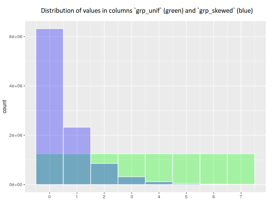
Distribution of record counts for the 2 partitioning columns
Partitioning examples using the interactive Spark shell
To show the partitioning and make example timings, we will use the interactive local Spark shell. We can run the Spark shell and provide it the needed jars using the --jars option and allocate the memory needed for our driver:
/usr/local/spark/spark-2.4.3-bin-hadoop2.7/bin/spark-shell \
  --jars /home/$USER/jars/mysql-connector-java-8.0.21/mysql-connector-java-8.0.21.jar \
  --driver-memory 7g
Now within the Spark shell, we can execute Scala expressions for three scenarios:
- no partitioning options provided (baseline)
- partitioning using the uniformly distributed column
- partitioning using the skewed column
After running these, we can compare the speed and see the benefit we gained by the different partitioning approaches versus the baseline.
// First, setup the data frame without partitioning
val reader_no_partitioning = spark.read.
  format("jdbc").
  option("url", "jdbc:mysql://localhost:3306/testdb").
  option("user", "rstudio").
  option("password", "pass").
  option("driver", "com.mysql.cj.jdbc.Driver").
  option("dbtable", "test_table")

val df_no_partitioning = reader_no_partitioning.load()
df_no_partitioning.cache().count()
df_no_partitioning.unpersist()

// Now use the skewed column to partition
val reader_partitioning_skewed = reader_no_partitioning.
  option("partitionColumn", "grp_skwd").
  option("numPartitions", 8).
  option("lowerBound", 0).
  option("upperBound", 4)
val df_partitioning_skewed = reader_partitioning_skewed.load()
df_partitioning_skewed.cache().count()
df_partitioning_skewed.unpersist()

// Now use the uniform column to partition
val reader_partitioning_unif = reader_no_partitioning.
  option("partitionColumn", "grp_unif").
  option("numPartitions", 8).
  option("lowerBound", 0).
  option("upperBound", 8)
val df_partitioning_unif = reader_partitioning_unif.load()
df_partitioning_unif.cache().count()
df_partitioning_unif.unpersist()
Comparing the performance of different partitioning options
Now let us look at how fast each of the read operations was. This is of course by no means a relevant benchmark for real-life data loads but can provide some insight into optimizing the partitioning. In our experience, the benefits of proper partitioning can be extremely relevant, especially with real-life use cases where the databases sit on external servers and support many concurrent connections.
First, let’s see the total time for the 3 options
- JobId 0 - no partitioning - total time of 2.9 minutes
- JobId 1 - partitioning using the
grp_skwdcolumn and 8 partitions - 2.1 minutes - JobId 2 - partitioning using the
grp_unifcolumn and 8 partitions - 59 seconds
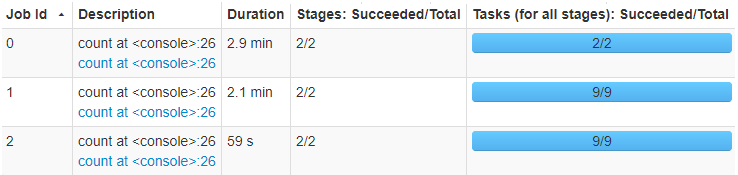
Timing of reading using different partitioning options
To understand better why the partitioning using the grp_unif column was so much faster, let us look at the performance per partition, with the partitioning using grp_skewed to the left the grp_unif to the right:
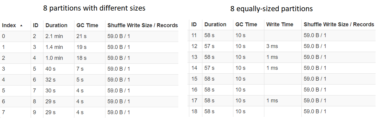
Investigating timing for each partition
We can see that the Durations for each of the partitions for grp_unif is almost identical, whereas for grp_skewed the longest time is much larger than the biggest time. This is heavily correlated with the sizes of each of the partitions, which points us toward our conclusion when looking at the actual implementation.
Understanding the partitioning implementation
The implementation of the partitioning within Apache Spark can be found in this piece of source code. The most notable single row that is key to understanding the partitioning process and the performance implications is the following:
val stride: Long = upperBound / numPartitions - lowerBound / numPartitionsIn combination with the while loop:
while (i < numPartitions) {
  val lBoundValue = boundValueToString(currentValue)
  val lBound = if (i != 0) s"$column >= $lBoundValue" else null
  currentValue += stride
  val uBoundValue = boundValueToString(currentValue)
  val uBound = if (i != numPartitions - 1) s"$column < $uBoundValue" else null
  val whereClause =
    if (uBound == null) {
      lBound
    } else if (lBound == null) {
      s"$uBound or $column is null"
    } else {
      s"$lBound AND $uBound"
    }
  ans += JDBCPartition(whereClause, i)
  i = i + 1
}
We can see that the data to be read is partitioned by splitting the values in the partitionColumn into numPartitions groups using the stride.
Based on this information, we can optimize the column that we choose for the partitioning as well as the values for upperBound and lowerBound such that the intervals for the values of partitionColumn will end up with roughly the same size.
In our example, the
- grp_unif column was purposefully generated such that this is the case with the most basic partitioning options, each partition having around 1.25 million records
- grp_skwd column had partitions with very different sizes, the biggest one with more than 6.3 million, whereas the smallest one with only around 9 thousand records
Setting up partitioning for JDBC via Spark from R with sparklyr
As we have shown in detail in the previous article, we can use sparklyr’s function spark_read_jdbc() to perform the data loads using JDBC within Spark from R. The key to using partitioning is to correctly adjust the options argument with elements named:
- numPartitions
- partitionColumn
- lowerBound
- upperBound
These are mapped one-to-one to the options as described above. Once we have done that, we pass the created options to the call to spark_read_jdbc() along with the other connection options in the options argument.
An oversimplified example of a full load could look like so:
# Setup jars and connect to Spark ----
jars <- dir("~/jars", pattern = "jar$", recursive = TRUE, full.names = TRUE)
config <- sparklyr::spark_config()
config$sparklyr.jars.default <- jars
config[["sparklyr.shell.driver-memory"]] <- "6G"
sc <- sparklyr::spark_connect("local", config = config)

# Create basic JDBC connection options ----
jdbcOpts <- list(
  user = "rstudio",
  password = "pass",
  server = "localhost",
  driver = "com.mysql.cj.jdbc.Driver",
  fetchsize = "100000",
  dbtable = "test_table",
  url = "jdbc:mysql://localhost:3306/testdb"
)

# Create the partitioning options ----
partitioningOpts <- list(
  numPartitions = 8L,
  partitionColumn = "grp_unif",
  lowerBound = 0L,
  upperBound = 8L
)

# Use the options combined to read a table ----
test_tbl <- sparklyr::spark_read_jdbc(
  sc,
  "test_table",
  options = c(jdbcOpts, partitioningOpts),
  smemory = FALSE
)

# Print a few records ----
test_tbl

# Disconnect ----
sparklyr::spark_disconnect(sc)
TL;DR, just tell me roughly how to partition
At the risk of oversimplifying and omitting some corner cases, to partition reading from Spark via JDBC, we can provide our DataFrameReader with the options:
option("partitionColumn", column_to_partition)
option("numPartitions", n)
option("lowerBound", x)
option("upperBound", y)
Such that when the stride is calculated as stride = y/n - x/n and the partitions are created by splitting the values of partitionColumn roughly like so:
Partition 1: Rows where column_to_partition ∈ <x, x+stride)
Partition 2: Rows where column_to_partition ∈ <x+stride, x+2*stride)
...
Partition n: Rows where column_to_partition ∈ <y-stride, y)
We try to set up the values of column_to_partition, n, x, y such that each of the created partitions is of roughly the same size.
Running the code in this article
If you have Docker available, running the following should yield a Docker container with RStudio Server exposed on port 8787, so you can open your web browser at http://localhost:8787 to access it and experiment with the code. The user name is rstudio and the password is as you choose below:
docker run -d -p 8787:8787 -e PASSWORD=pass jozefhajnala/jozefioReferences
- A guide to retrieval and processing of data from relational database systems using Apache Spark and JDBC with R and sparklyr
- JDBC To Other Databases in Spark documentation
- Discussion on the JDBC partitioning topic at StackOverflow
- Tips for using JDBC in Apache Spark SQL by Radek Strnad
- Class DataFrameReader as Spark’s Scala API Doc
- DataFrameReader implementation at GitHub